Table Of Content

A farmer possesses five plots of land where he wishes to cultivate corn. He wants to run an experiment since he has two kinds of corn and two types of fertilizer. Moreover, he knows that his plots are quite heterogeneous regarding sunshine, and therefore a systematic error could arise if sunshine does indeed facilitate corn cultivation. In that sense, Latin Square designs are useful building blocksof more complex designs, see for example Kuehl (2000).
Unit Requirements
The design is balanced having the effect that our usual estimators andsums of squares are “working.” In R, we would use the model formulay ~ Block1 + Block2 + Treat. We cannot fit a more complex model, includinginteraction effects, here because we do not have the corresponding replicates. To estimate the efficiency that was gained by blocking (relative to completely randomized design). For example you might have 5 levels of a factor, but when you split your block into plots, you can only create 3 plots. The yield of oats from a split-plot field trial using three varieties and four levels of manurial treatment. The experiment was laid out in 6 blocks of 3 main plots, each split into 4 sub-plots.
Construction of symmetric paired choice experiments: minimising runs and maximising efficiency Humanities and ... - Nature.com
Construction of symmetric paired choice experiments: minimising runs and maximising efficiency Humanities and ....
Posted: Tue, 03 Oct 2023 07:00:00 GMT [source]
Balanced Incomplete Block Design (BIBD)
The number of rows and columns has to correspond to the number of treatment levels. So, if we have four treatments then we would need to have four rows and four columns in order to create a Latin square. This gives us a design where we have each of the treatments and in each row and in each column. If the structure were a completely randomized experiment (CRD) that we discussed in lesson 3, we would assign the tips to a random piece of metal for each test. In this case, the test specimens would be considered a source of nuisance variability.
Chapter 7 Improving Precision and Power: Blocked Designs
We already know how to deal with these variables by adding them to the model, but there are experimental designs where we must be careful because the experimental treatments are nested. The idea of a latin square can be extended to more than two blocking factors; with three factors, such designs are called graeco-latin squares. Ok, with this scenario in mind, let's consider three cases that are relevant and each case requires a different model to analyze. The cases are determined by whether or not the blocking factors are the same or different across the replicated squares.
The ANOVA for Randomized Complete Block Design (RCBD)
For units to be considered in "residence," you must be registered in courses on the Berkeley campus as a student in the College of Letters & Science. Most students automatically fulfill the residence requirement by attending classes here for four years, or two years for transfer students. In general, there is no need to be concerned about this requirement, unless you go abroad for a semester or year or want to take courses at another institution or through UC Extension during your senior year. In these cases, you should make an appointment to meet an adviser to determine how you can meet the Senior Residence Requirement. Students should apply in the semester they will complete their prerequisites. For applicants with prerequisites in progress, applications will be reviewed after the grades for all prerequisites are available, 2-3 weeks after finals.
If you look at all possible combinations in each row, each treatment pair occurs only one time. If you look at how we have coded data here, we have another column called residual treatment. For the first six observations, we have just assigned this a value of 0 because there is no residual treatment. But for the first observation in the second row, we have labeled this with a value of one indicating that this was the treatment prior to the current treatment (treatment A). In this way the data is coded such that this column indicates the treatment given in the prior period for that cow.
Significance Level
We want a design with 3 blocking factors; machine, operator, and day of the week. The choice of case depends on how you need to conduct the experiment. If you are simply replicating the experiment with the same row and column levels, you are in Case 1. If you are changing one or the other of the row or column factors, using different machines or operators, then you are in Case 2. If both of the block factors have levels that differ across the replicates, then you are in Case 3.
2 The Randomized Complete Block Design

So you can analyze the resulting data, but now should reduce your error degrees of freedom by one. In any event, these are all approximate methods, i.e., using the best fitting or imputed point. The test on the block factor is typically not of interest except to confirm that you used a good blocking factor. Variability between blocks can be large, since we will remove this source of variability, whereas variability within a block should be relatively small. In this example we wish to determine whether 4 different tips (the treatment factor) produce different (mean) hardness readings on a Rockwell hardness tester. The treatment factor is the design of the tip for the machine that determines the hardness of metal.
3.2 Defining a Balanced Incomplete Block Design
Nesting them enables estimation of their respective variance components, while crossing leads to row-column designs that control for two sources of variation simultaneously. A typical example of a non-random classification factor is the sex of an animal. The Hasse diagrams in Figure 7.6 show an experiment design to study the effects of our three drugs on both female and male mice.
If the blocks aren't homogeneous, their variability will not be less than that of the entire sample. In that situation, randomized block design can decreases the statistical power and thus be worse than a simple single-factor between-subjects randomized design. Again, your best bet on finding an optimal number of blocks is from theoretical and/or empirical evidences. First, we might consider replicating columns while keeping the rows, using \(rk\) column factor levels instead of \(k\). The same logic applies to keeping columns and replicating rows, of course. The two experiments in Figure 7.14B illustrate this design for a two-fold replication of the \(3\times 3\) latin square, where we use six litters instead of three, but keep using the same three cages in both replicates.
Typical block factors are location (see example above), day (if an experiment isrun on multiple days), machine operator (if different operators are needed forthe experiment), subjects, etc. Ideally I wouldn’t have to do the averaging over the nested observations and we would like to not have the misleading p-values for the plots. To do this, we only have to specify the nesting of the error terms and R will figure out the appropriate degrees of freedom for the covariates. Because this is an orthogonal design, the sums of squares doesn’t change regardless of which order we add the factors, but if we remove one or two observations, they would.
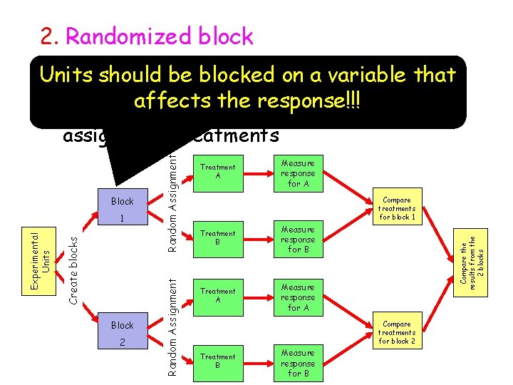
In contrast to a randomized complete block design, we cannot increase the number of blocks to increase the replication. With two levels of Sex fixed, we instead need to increase the experiment size by using multiple mice of each sex for each drug. Since Sex and Drug are fixed, so is their interaction, and all fixed factors are tested against the same error term from (Mouse). A simple yet powerful design is the randomized complete block design (RCBD), where each block has as many units as there are treatments, and we randomly assign each treatment to one unit in each block.
To address nuisance variables, researchers can employ different methods such as blocking or randomization. Blocking involves grouping experimental units based on levels of the nuisance variable to control for its influence. Randomization helps distribute the effects of nuisance variables evenly across treatment groups. Nesting blocking factors allows us to replicate already blocked designs, to combine several properties for grouping, and to disentangle the variance components of different levels of grouping. We consider only designs with two nested blocking factors, but our discussion directly extends to longer chains of nested factors. In contrast to a two-way ANOVA with factorial treatment structure, we cannot simplify the analysis to a one-way ANOVA with a single treatment factor with \(b\cdot k\) levels.


No comments:
Post a Comment